Part distortion during machining is a significant problem in many industries, particularly where rigorous dimensional tolerances are required. Distortion of finished parts can lead to significant economic loss and should be managed for effective design and production. This case study demonstrates some of the basic concepts related to the impact of residual stress on part distortion during machining. A representative problem is defined, and a model is used to estimate part distortion due to machining of raw material containing bulk residual stress.
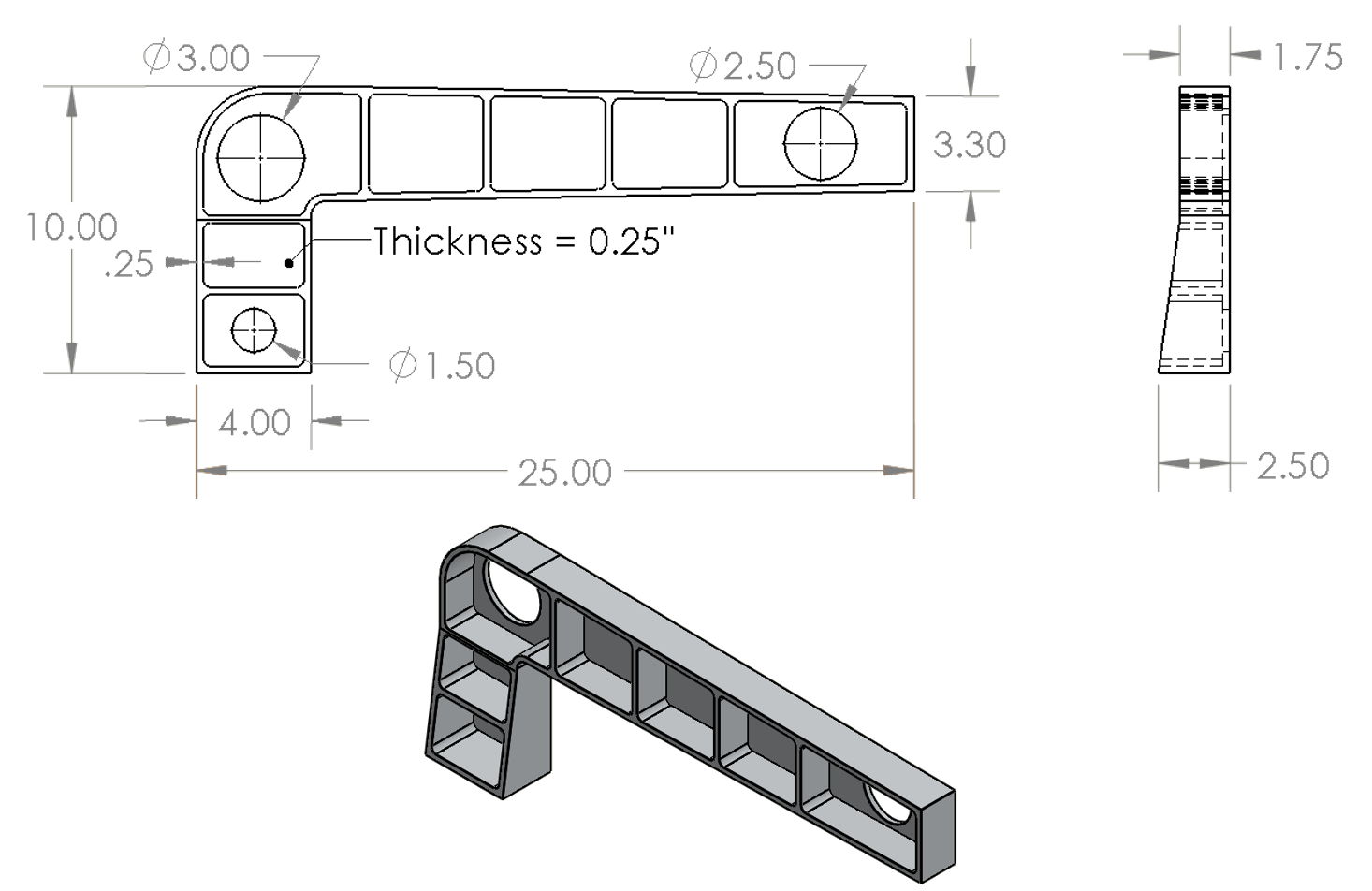
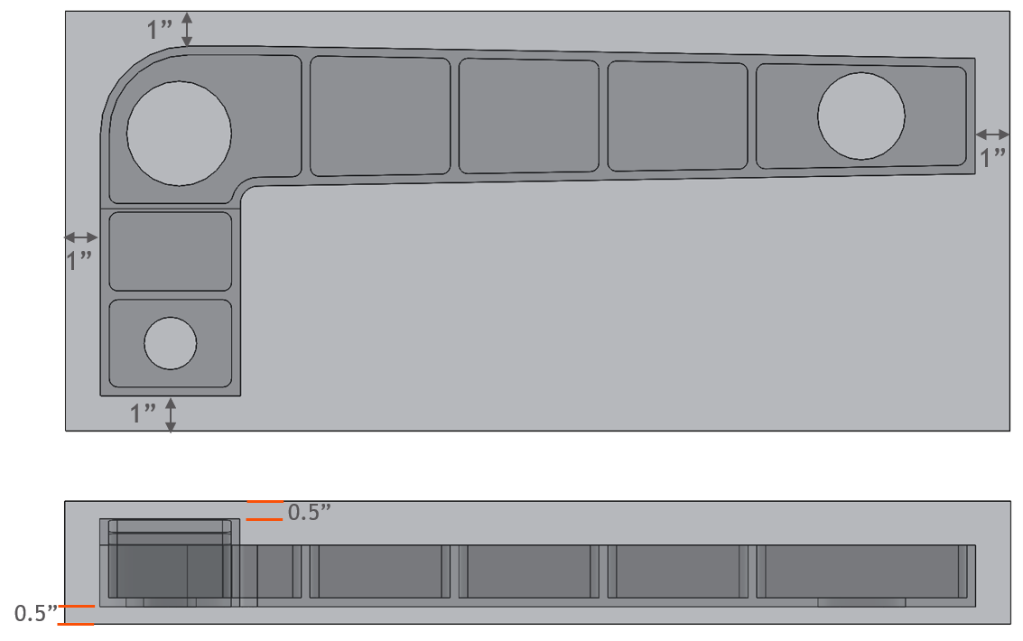
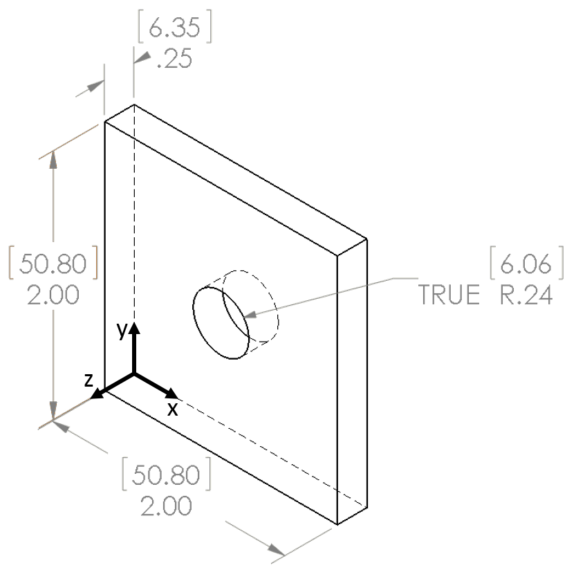
This study considers a 304.8 x 203.2 x 12.7 mm (12.0 x 8.0 x 0.5 inch) aluminum plate as the starting raw material for the analysis. From the plate an example part will be machined that has the same in-plane dimensions as the starting plate (304.8 mm x 203.2 mm) and includes a 2.54 mm (0.1 inch) thick frame around a 2.54 mm (0.1 inch) thick web.
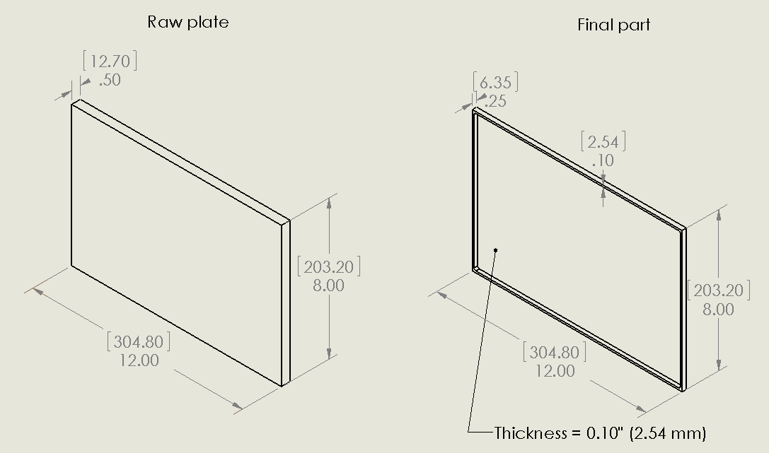
Raw plate and final part geometry. Non-bracketed dimensions are in inches and bracketed dimensions are in mm.
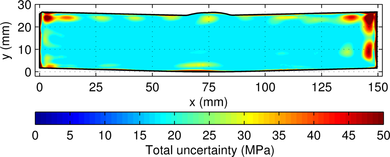
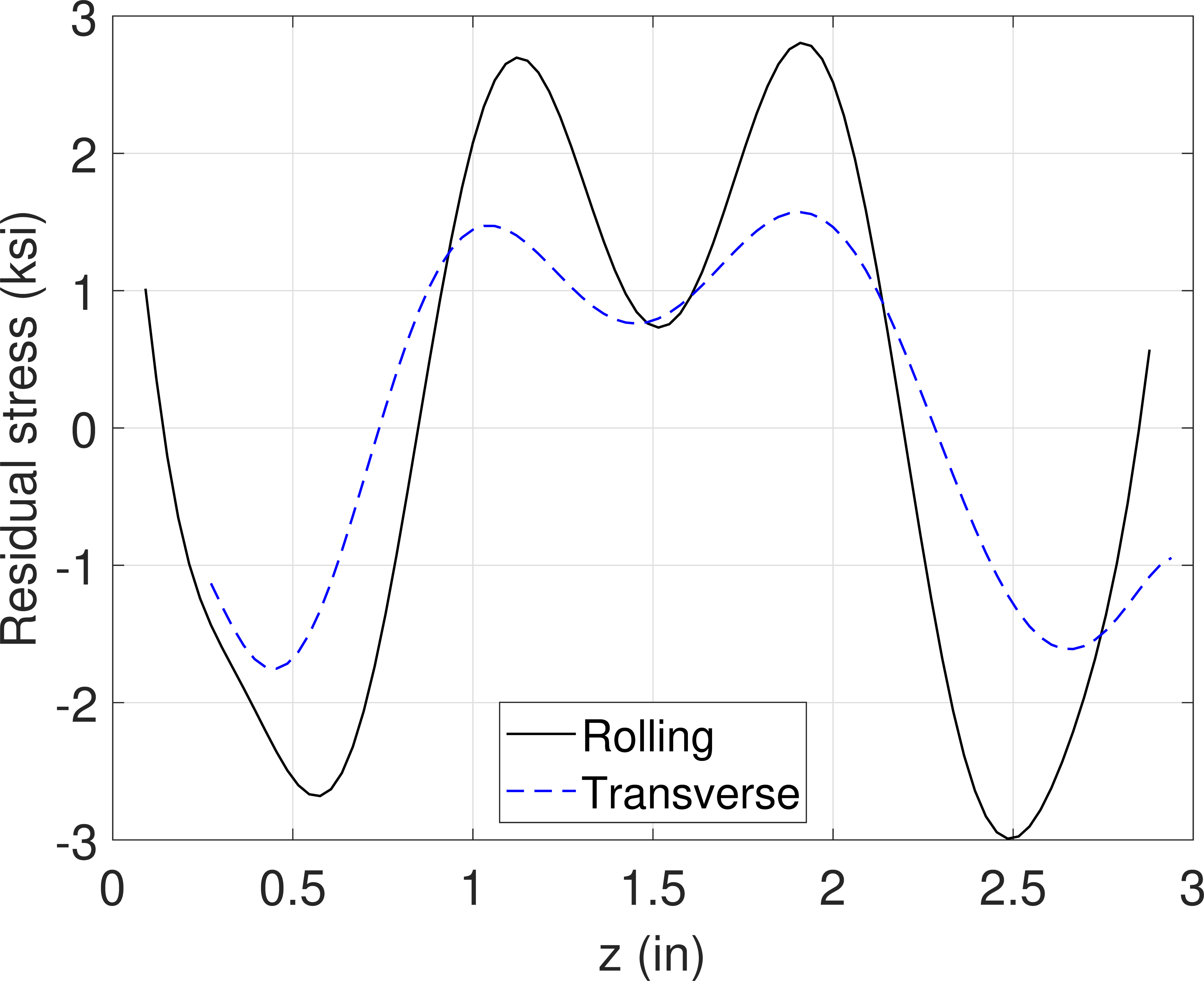
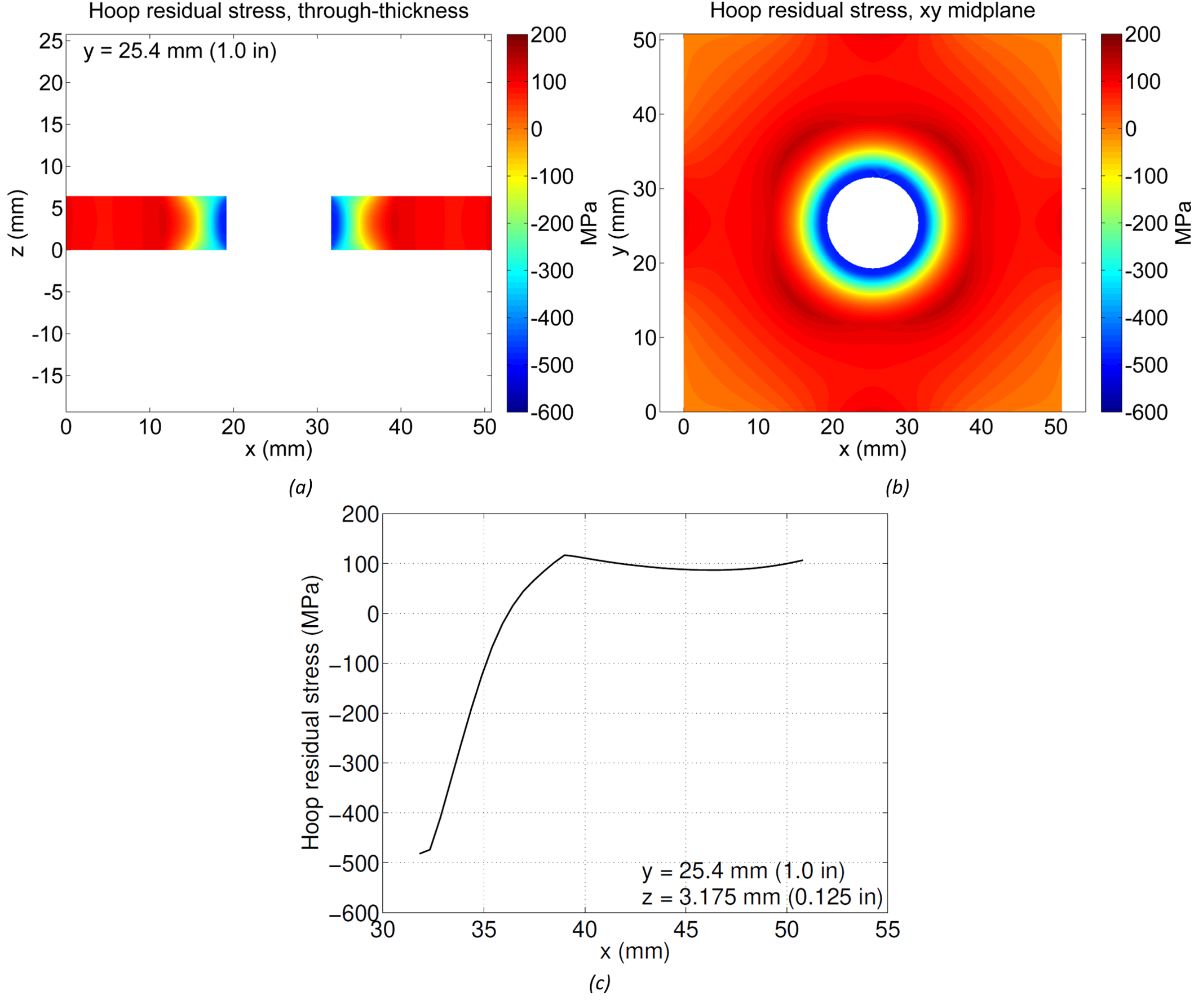
Aluminum plate is often stress relieved by stretching, and typically exhibits low levels of residual stress post-stress relief. For the sake of this analysis, the raw material is assumed to have the residual stress distribution shown in Figure 2a (similar to the residual stress measured by Prime and Hill [1]). The residual stress values are low compared to the yield strength of the material, ranging from about -20 to 20 MPa (-3 to 3 ksi).
In addition to the bulk residual stress present in the raw material, the machining process also induces stress. The machining-induced residual stress assumed for this demonstration is shown in Figure 2b, and exhibits a typical distribution with compressive residual stress near the machined surface that spans over a thin layer (0.2 mm) before it reaches magnitudes near zero. The peak compressive residual stress at the machined surface is -50 MPa (~ 7.3 ksi). The bulk residual stress in Figure 2a is assumed to be present in the raw plate for the analysis, while the machining-induced residual stress in Figure 2b is applied locally to the machined surfaces.
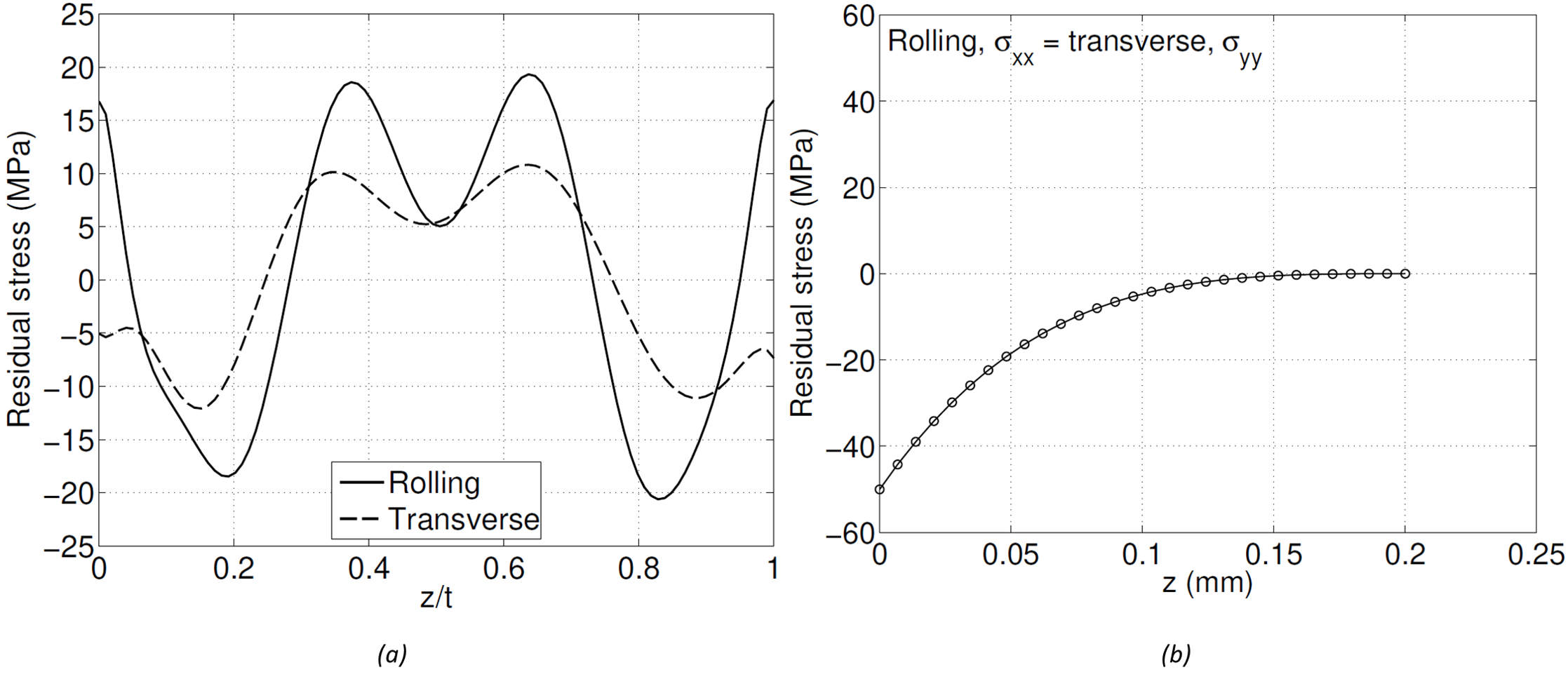
(a) Bulk residual stress (similar to [1] along rolling and transverse direction, (b) idealized machining induced residual stress
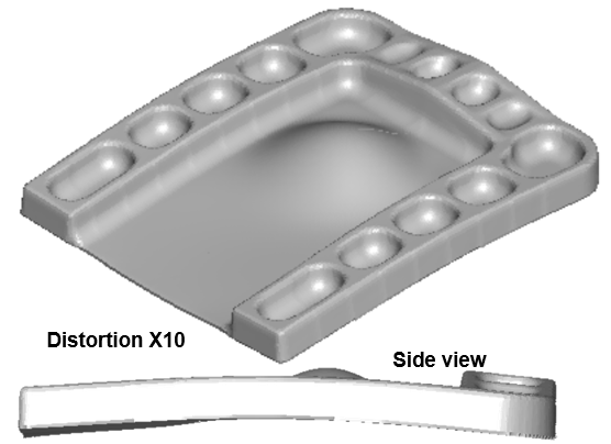
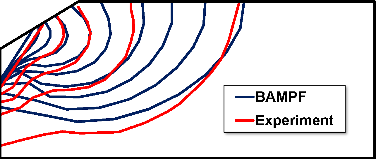
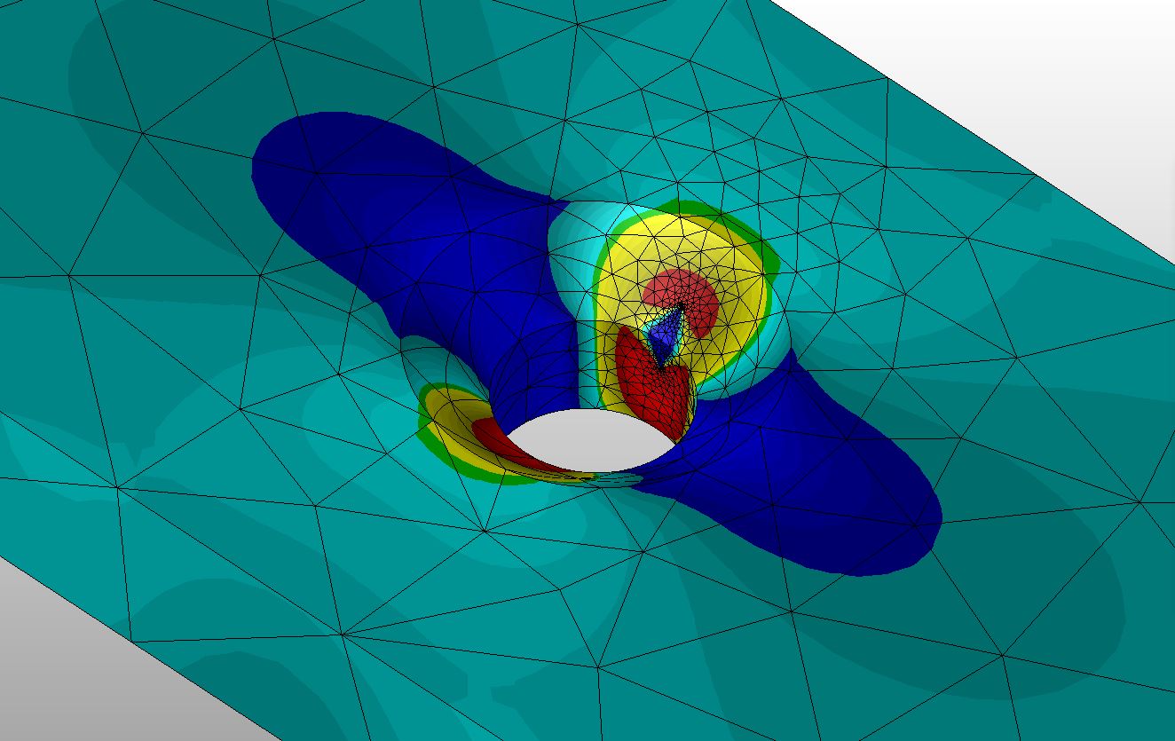
A finite element model including the bulk and machining-induced residual stresses was used to predict the distortion of the finished part. The model is elastic and superposes bulk and machining residual stress to provide an equilibrium solution. Figure 3a shows the deformed shape (using a magnification factor of 30 to better illustrate the deformation). The displacement pattern shows bowing of the finished part with respect to its intended shape, with positive displacements near the center. A 2D map of the displacement of the bottom surface of the finished part is shown in Figure 3b. Line plots along the x direction at y = 101.6 mm and along the y direction at x = 152.4 mm are shown in Figure 3c. The distortion range is approximately 1.4 mm. It is important to note that even though the bulk residual stress in the raw material is low (about 5% of the yield strength), it still has potential to cause significant distortion in finished parts, as illustrated here.
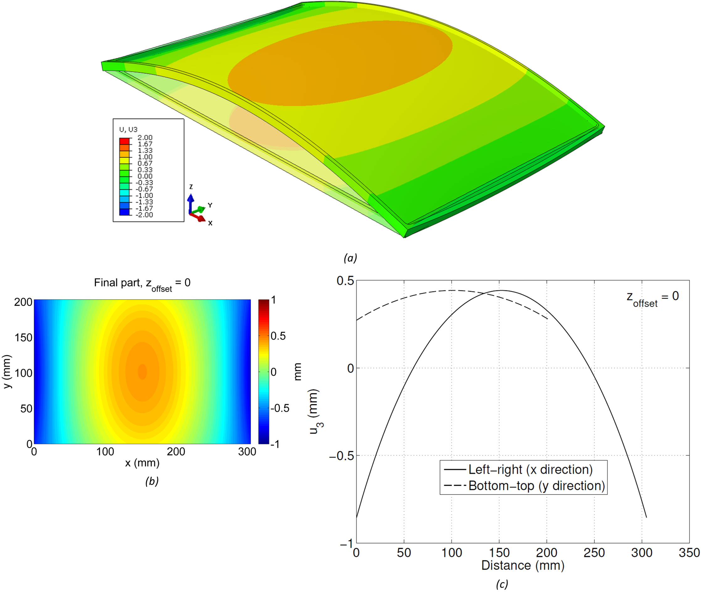
(a) Undeformed/deformed 3D shape of final part with zoffset = 0, (b) 2D map of leveled displacement of bottom surface, (c) line plots along paths from left-right and bottom-top
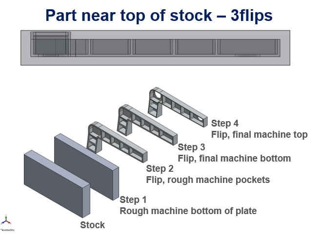
Since the raw plate is thicker than the final part, the final part can be extracted from different positions through the thickness of the raw plate (e.g., Figure 4). The position from within the raw plate that the final part is removed from can have a significant impact on the distortion (due to the different bulk residual stress levels at different locations through the thickness). The position is defined by an offset distance from the bottom surface of the raw plate, zoffset. In the first example, the zoffset = 0, i.e., the bottom surface of the final part is aligned with the bottom surface of the raw plate (z = 0).
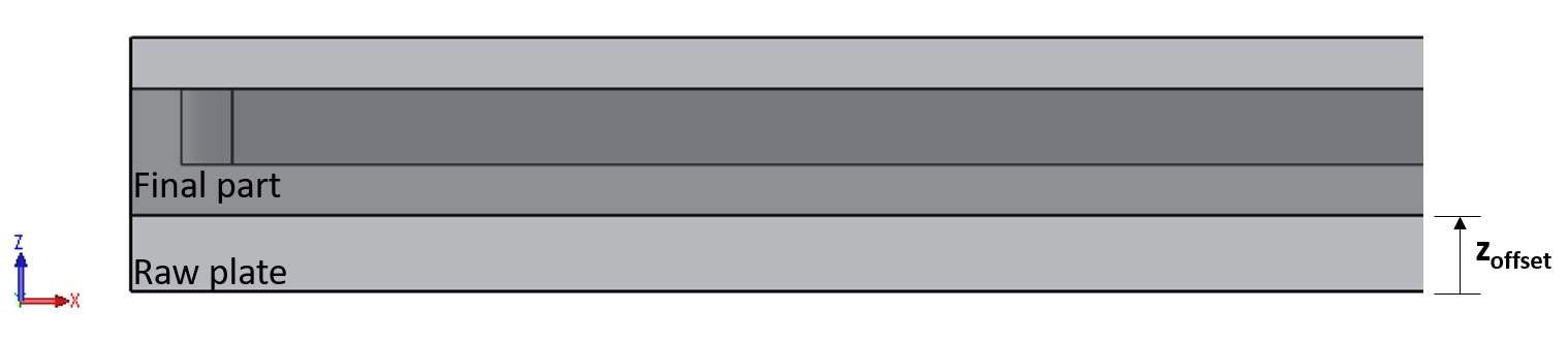
Location of machining of baseline/final part within the raw plate
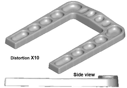
The model used here can be modified to consider different part placements within the raw material in a straightforward manner. A significantly different result was obtained considering zoffset = 2.54 mm (0.1inch), which is shown in Figure 5. An opposite pattern of distortion is observed in Figure 5a compared to the case where zoffset = 0 (Figure 3a). The 2D map shown in Figure 5b shows displacements that range from 1.1 mm to -0.6 mm. Figure 5c shows the displacement along the left-right and bottom-top paths, and includes the results obtained with zoffset = 0 for comparison. Compared to zoffset = 0, zoffset = 2.54 mm exhibits displacement along the x direction that ranges from positive-negative-positive values and with higher magnitudes. The displacement along the y direction is similar for both offsets, but have opposite signs.
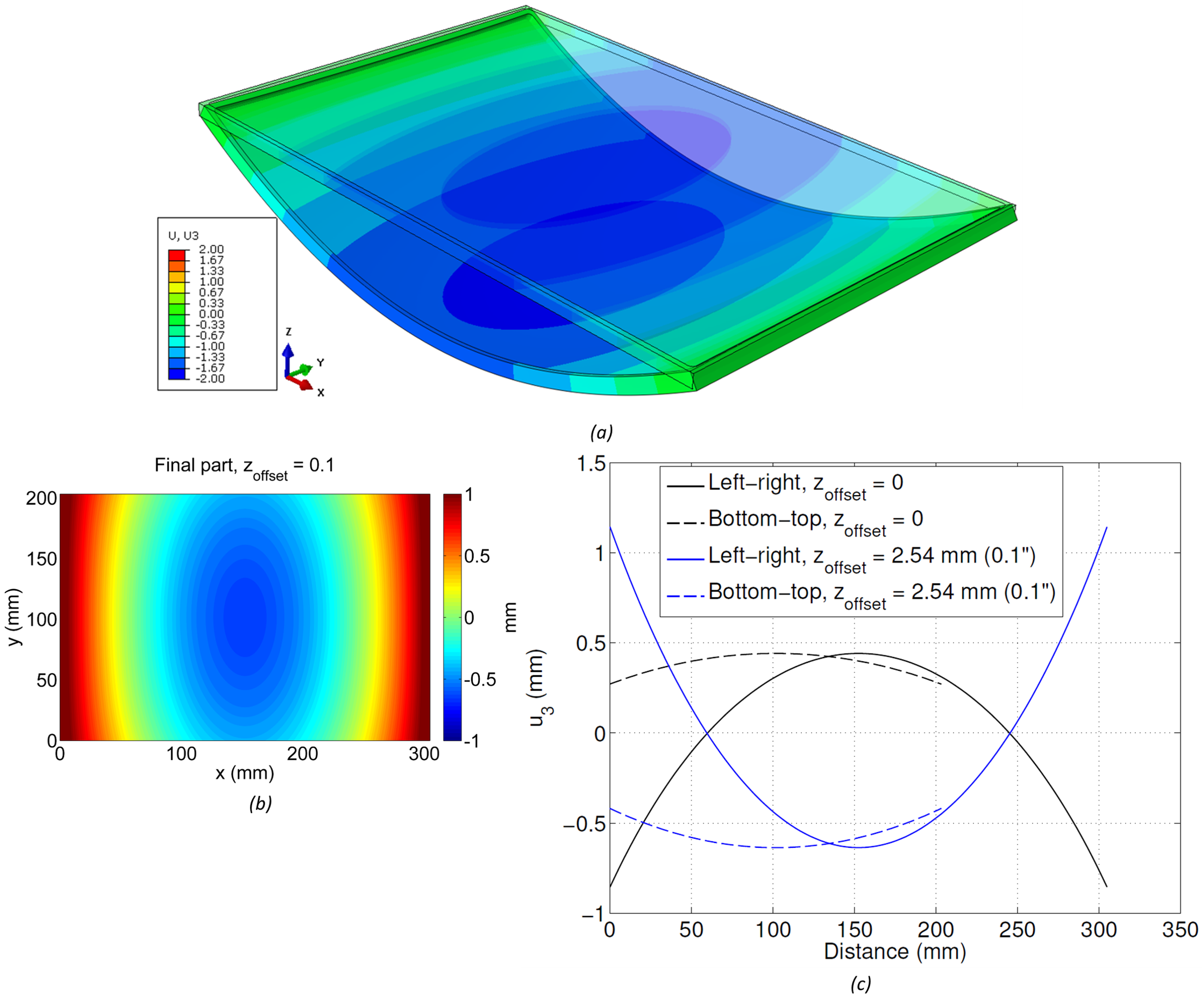
(a) Undeformed/deformed 3D shape of final part with zoffset = 2.54 mm (0.1inch), (b) 2D map of leveled displacement of bottom surface, (c) line plots along paths from left-right and bottom-top comparing zoffset = 0 and 2.54 mm
Another aspect that influences the part distortion is the thickness of the web of the large pocket. The previous results considered a thickness of 2.54 mm (0.1inch), as illustrated in the final part drawing in Figure 1. Reducing the thickness to 0.635 mm (0.025inch) and considering the zoffset = 0 configuration causes significant changes in the results, as observed in Figure 6. A similar pattern of distortion is observed in Figure 6a and Figure 6b compared to Figure 3a and Figure 3b, however the magnitudes of displacement are significantly lower. A line plot comparing the results obtained with both thicknesses is shown in Figure 6c. Overall, the model with reduced thickness (red lines) provides lower displacement magnitudes along both paths (left-right and bottom-top) compared to the initial model with 2.54 mm thickness, and exhibits peak displacement that is lower by about 50%.
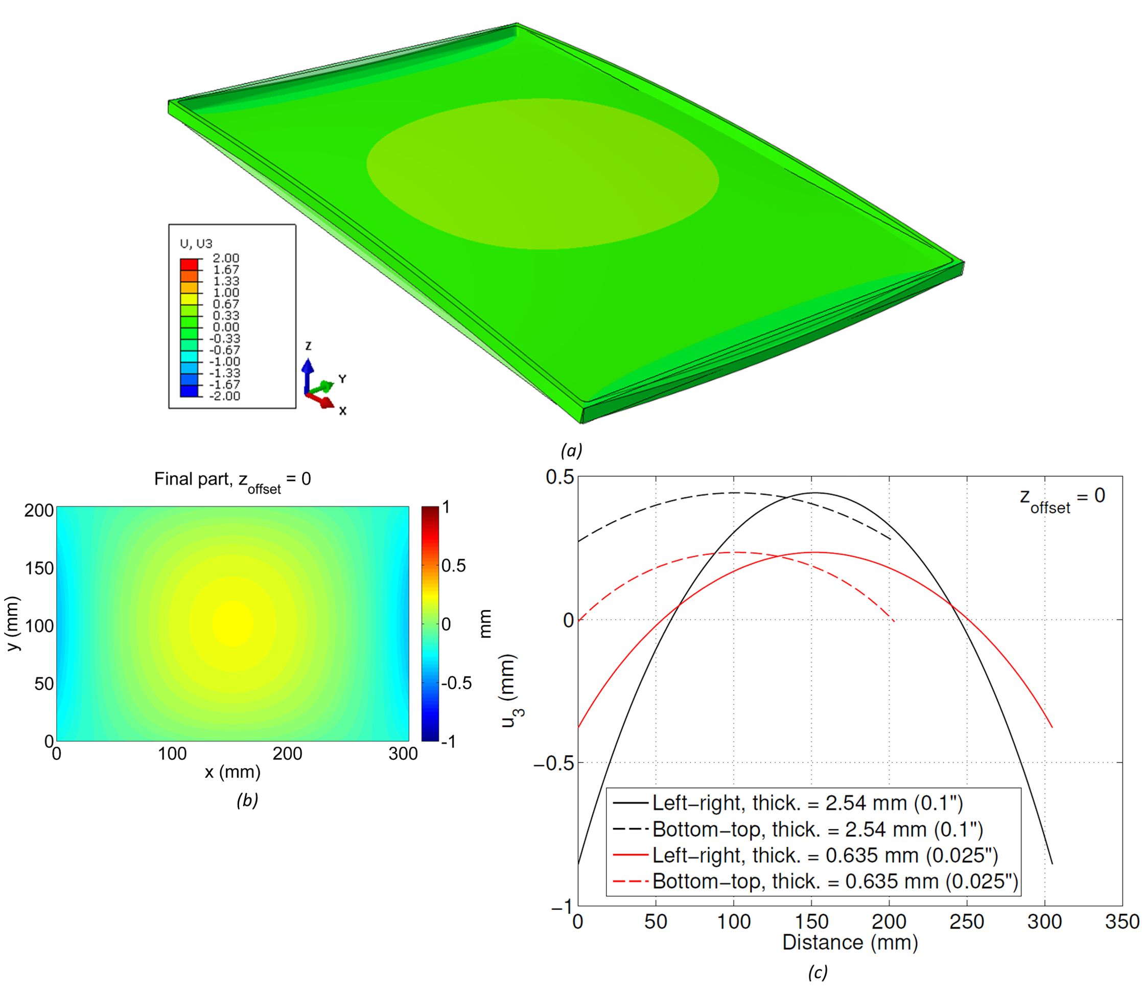
(a) Undeformed/deformed 3D shape of final part with zoffset = 0, (b) 2D map of leveled displacement of bottom surface, (c) line plots along paths from left-right and bottom-top comparing thickness = 0.635 mm (0.025inch) and 2.54 mm (0.1inch)
This case study provided an example problem for the estimation of part distortion due to residual stress release from machining, considering a typical bulk residual stress distribution and machining-induced residual stress distribution. The results show significant part distortion, even though the considered bulk residual stress had very low magnitude compared to the yield strength of the material. The results also show that part distortion varies significantly depending on the machining location within the raw stock material.
For more information concerning this case study or any of the residual stress measurement techniques employed at Hill Engineering, feel free to contact us.
[1] M. B. Prime and M. R. Hill, “Residual stress, stress relief, and inhomogeneity in aluminum plate,” Scripta Materialia, pp. 77-82, 2002.